Computer Face Recognition
The Bottom-up Stimulus for Computers in Face Recognition
The pixel is the unit of measure for a digital image.
Colors can be represented in hex, RGB, gray-scale intensity and other identification schemes.
| Base | Red | Green | Blue |
|---|---|---|---|
| Decimal | 255 | 0 | 0 |
| Octal (8) | 377 | 0 | 0 |
| Hex (16) | FF | 00 | 00 |
| Binary | 1111 1111 | 0000 0000 | 0000 0000 |
Pixels are assembled in a grid system. Each one has coordinates. Each pixel is specified by its position within the grid system as identified by (x-axis, y-axis) using integers.
Face detection is a two class problem where we have to decide if there is a face or not in a picture. Here, we introduce four different general approaches:
These are rule-based methods. They try to capture our knowledge of faces, and translate them into a set of rules. It’s easy to guess some simple rules. For example, a face usually has two symmetric eyes, and the eye area is darker than the cheeks. Facial features could be the distance between eyes or the color intensity difference between the eye area and the lower zone.
The big problem with these methods is the difficulty in building an appropriate set of rules. There could be many false positives if the rules were too general. On the other hand, there could be many false negatives if the rules were too detailed.
Algorithms that try to find invariant features of a face despite it’s angle or position. The idea is to overcome the limits of our instinctive knowledge of faces.
Template matching methods try to define a face as a function. We try to find a standard template of all the faces. Different features can be defined independently. For example, a face can be divided into eyes, face contour, nose and mouth. Also a face model can be built by edges. A face can also be represented as a silhouette. Other templates use the relation between face regions in terms of brightness and darkness. These standard patterns are compared to the input images to detect faces.
This approach is simple to implement, but it’s inadequate for face detection. It cannot achieve good results with variations in pose, scale and shape.
A template matching method whose pattern database is learnt from a set of training images.
In general, appearance-based methods rely on techniques from statistical analysis and machine learning to find the relevant characteristics of face images. Some appearance-based methods work in a probabilistic network. An image or feature vector is a random variable with some probability of belonging to a face or not. Another approach is to to define a discriminant function between face and non-face classes.
TLDR: This is a template matching algorithm. Taking a gray-scale image, we represent the entire image by using arrows, at each pixel, to point towards the direction that the image is getting darker. And then we can see if the pattern of arrows resembles a face or not.
Taking the gray-scale picture above, we can draw an arrow at the marked pixel showing in which direction the image is getting darker.
If you repeat that process for every single pixel in the image, you end up with every pixel being replaced by an arrow. These arrows are called gradients and they show the flow from light to dark across the entire image:
By only considering the direction that brightness changes, we reduces the influence of different illumination.
Saving the gradient for every single pixel gives us way too much detail. We end up missing the forest for the trees. It would be better if we could just see the basic flow of lightness/darkness at a higher level so we could see the basic pattern of the image
The original image is turned into a HOG representation that captures the major features of the image regardless of image brightnesss.
To find faces in this HOG image, all we have to do is find the part of our image that looks the most similar to a known HOG pattern that was extracted from a bunch of other training faces:
This feature extraction process can be defined as the procedure of extracting relevant information from a face image. This information must be valuable to the later step of identifying the subject with an acceptable error rate. The feature extraction process must be efficient in terms of computing time and memory usage. The output should also be optimized for the classification step.
The performance of a classifier depends on the amount of sample images, number of features and classifier complexity.
Rationale for reducing dimensionality:
Ultimately, the number of features must be carefully chosen. Too less or redundant features can lead to a loss of accuracy of the recognition system.
Features are extracted from the face images, then a optimum subset of these features is selected. It aims to select a subset of the extracted features that cause the smallest classification error. Dimension reduction method can be embedded in the selection method.
TLDR: This feature extraction algorithm uses the numerical method of principle component analysis (PCA) to select a representative set of features that, when combined linearly, best describes faces in a low dimension.
If we take small images of faces as the feature vector, without detecting local features, then, for example, a 100x100 image is considered a 10000 dimensional feature vector. Each of these vectors are a location in a 10000 dimensional vector space. Practically any vector in this space is a 100x100 image.
As these are vectors just like any other vector, we can compute difference vectors, average vectors, sum of vectors etc. The difference of two face-vectors is obviously not a face, it is just a difference image.
If we can find a smaller set of basis vectors that can be used to reconstruct the vectors in the dataset, we can represent them in a more compact way. This process of finding a smaller set of basis vectors to represent the data is called dimensionality reduction. For the space of faces this means: we need to find some set of vectors (corresponding to images) that can be used to mix any face image. If we can manage to find such a set, we will have a much more compact representation of faces.
The Principal Component Analysis is the tool to find this subspace, find a new set of basis vectors that can be used to mix any data vector.
Eigenfacesare the significant eigenvectors of the face dataset. Using the eigenfaces, which are really images, any face image can be mixed using a simple linear combination. This means we can represent any face with weights of the eigenfaces.
While some eigenfacesseem to correspond to real features such as beard or glasses, in general eigenfacesare not faces. They are just difference images used to recreate any face in the dataset.
First image is the average face, the others are the eigenfaces.
If the eigenfacesare chosen properly, eg: we include all eigenfaces with larger eigenvalues, any face in the dataset can be reconstructed by a linear combination of the eigenfaces. To come up with these weights for a real face image, we simply need to multiply this 10000 dimensional input vector by a rotation matrix and drop all components with indices greater than K (the number of features we want to keep).
x is an N dimensional feature vector. v1, v2,..., vk are eigenfaces.
x = x_avg + a1v1 + a1v2 + ... + akvk
The eigenfacesneed to be computed only once, and then all faces in the database can be represented by a set of weights. This is a much more compact representation.
Then, to verify if there is a face on a new image we simply need to compute the reconstruction with eigenfaces and check if the reconstruction matches the original image. If it does, we are likely dealing with a face image.
To identify the face we need to find the closest weight-vector in the database and see if they are closed then some distance threshold.
Appearance-based face recognition algorithms use a wide variety of classification methods. Sometimes two or more classifiers are combined to achieve better results. On the other hand, most model-based algorithms match the samples with the model or template.
Then, a learning method is can be used to improve the algorithm - supervised, unsupervised or semi-supervised. Unsupervised learning is the most difficult approach, as there are no tagged examples. However, many face recognition applications include a tagged set of subjects. Consequently, most face recognition systems implement supervised learning methods. There are also cases where the labeled data set is small. Sometimes, the acquisition of new tagged samples can be infeasible. Therefore, semi-supervised learning is required.
One way or another, classifiers have a big impact in face recognition. Classification methods are also generally used in many areas like data mining, finance, signal decoding, voice recognition, natural language processing or medicine. 2 concepts that are key in building a classifier - similarity and probability.
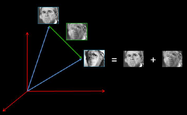
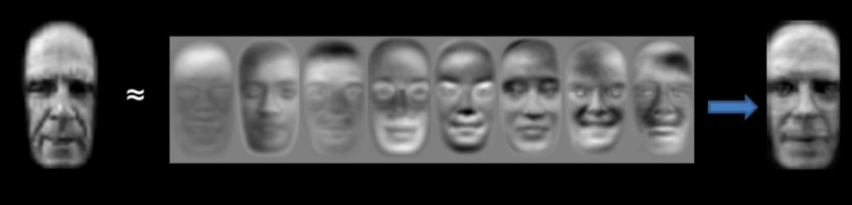
where wi are the face classes and Z an image in a reduced PCA space.
Combining the idea of face detection and feature extraction ideas above, we see a wide variety of comprehensive face recognition algorithms applied in computer vision. We can summarize them into three different broad categories: template matching, statistical approach and neural network. The examples above corresponds to ideas within template matching and statistical category. Here, we want to show an example of how neural network face recognition algorithm works.
The measurements that seem obvious to us humans (like eye color) don’t really make sense to a computer looking at individual pixels in an image. Researchers have discovered that the most accurate approach is to let the computer figure out the measurements to collect itself. Deep learning does a better job than humans at figuring out which parts of a face are important to measure.
The solution is to train a Deep Convolutional Neural Network to generate a number of different measurements for each face.
The training process works by looking at 3 face images at a time:
Then the algorithm looks at the measurements it is currently generating for each of those three images. It then tweaks the neural network slightly so that it makes sure the measurements it generates for #1 and #2 are slightly closer while making sure the measurements for #2 and #3 are slightly further apart.
Machine learning people call these measurements of each face an embedding. The idea of reducing complicated raw data like a picture into a list of computer-generated numbers comes up a lot in machine learning (especially in language translation).
This process of training a convolutional neural network to output face embeddings requires a lot of data and computer power. With days of continuous training to get good accuracy, we will have a trained network that can generate measurements for any face, even ones it has never seen before! The network should generate nearly the same numbers when looking at two different pictures of the same person.
This last step is actually the easiest step in the whole process. All we have to do is find the person in our database of known people who has the closest measurements to our test image. And you can do that by using any basic machine learning classifier (eg: nearest neighbor, or the classifiers mentioned above, etc.).